Variance and Bias (분산과 편향)

Introduction

In the realm of machine learning, two fundamental concepts play a crucial role in determining the performance and reliability of predictive models: bias and variance. These concepts are not just theoretical constructs but have significant practical implications for anyone working with predictive analytics.

Bias refers to the error introduced by approximating a real-world problem with a simplified model, while variance is the error due to the model's sensitivity to fluctuations in the training data. Understanding these concepts is key to addressing the central challenge in supervised learning: the bias-variance tradeoff.

The importance of bias and variance in machine learning cannot be overstated. They guide us in:

1. Model Selection: Choosing the most appropriate model for a given problem.
2. Performance Optimization: Tuning model parameters for optimal performance.
3. Error Diagnosis: Identifying whether a model is underfitting or overfitting.
4. Data Collection Strategies: Informing decisions about data collection and feature relevance.
5. Setting Realistic Expectations: Guiding discussions about model limitations and potential improvements.

What is Bias?

Bias, in the context of machine learning, refers to the error introduced by approximating a real-world problem, which may be extremely complicated, by a much simpler model. It's a measure of how far off in general a model's predictions are from the correct values. In essence, bias is the difference between the expected (or average) prediction of our model and the correct value which we are trying to predict.

High bias is typically associated with simpler models that make strong assumptions about the data. These models are said to "underfit" the data, meaning they fail to capture important patterns or relationships. Examples of high-bias models include:

1. Linear regression for non-linear relationships
2. Naive Bayes classifiers that assume feature independence
3. Decision trees with very shallow depth

On the other hand, low bias models are more flexible and can capture complex patterns in the data. These might include:

1. Deep neural networks
2. Random forests with many trees
3. Support Vector Machines with non-linear kernels

It's important to note that while low bias sounds desirable, it often comes at the cost of higher variance, which we'll discuss in the next section.

How bias affects model predictions can be seen in several ways:

1. Systematic Error: High bias models tend to make systematic errors. They consistently miss certain patterns or relationships in the data.

2. Underfitting: Biased models underfit the training data, meaning they perform poorly not just on new, unseen data, but also on the data they were trained on.

3. Simplistic Predictions: High bias models often make overly simplistic predictions that fail to capture the nuances of the problem.

4. Poor Generalization: While low bias models can capture complex patterns, extremely low bias can lead to poor generalization if not balanced with appropriate variance control.

To illustrate this concept, let's consider a simple example. Imagine we're trying to predict house prices based on their size. Our true relationship might be quadratic:

price = 100,000 + 100 * size + 0.1 * size^2

But our model is a simple linear regression:

predicted_price = b0 + b1 * size

No matter how we adjust b0 and b1, our model will always have some bias because it can't capture the quadratic relationship. It will systematically underestimate prices for very small and very large houses, while overestimating for medium-sized houses.

Recognizing and addressing bias is crucial for developing effective machine learning models. High bias can lead to models that are too simplistic to be useful, while extremely low bias can lead to overfitting if not properly managed.

What is Variance?

Variance, in the context of machine learning, refers to the model's sensitivity to fluctuations in the training data. It measures how much the predictions of a model would change if it were trained on a different dataset. High variance models are those that vary significantly in their predictions when trained on different subsets of the data.

To understand variance intuitively, imagine fitting a complex polynomial to a dataset with some noise. The model might fit the training data perfectly, capturing not just the underlying trend but also the random noise. However, if we were to collect a new dataset and fit the same model, the resulting polynomial might look quite different, as it would be fitting to a different set of random noise. This sensitivity to the specific training data is what we call variance.

High variance is typically associated with complex models that have a large number of parameters relative to the size of the training data. These models are said to "overfit" the data, meaning they capture not just the underlying patterns but also the noise in the training set. Examples of models prone to high variance include:

1. Decision trees with many levels (deep trees)
2. K-Nearest Neighbors with small K
3. Neural networks with many layers and neurons

On the other hand, low variance models are more stable and less sensitive to fluctuations in the training data. These might include:

1. Linear regression
2. Logistic regression
3. Decision trees with few levels (shallow trees)

How variance impacts model generalization is crucial to understand:

1. Overfitting: High variance models tend to overfit the training data. They perform extremely well on the training set but poorly on new, unseen data.

2. Instability: Models with high variance are unstable. Small changes in the training data can lead to large changes in the model's predictions.

3. Poor Generalization: While high variance models can capture complex patterns in the training data, they often fail to generalize well to new data.

4. Noise Sensitivity: High variance models are sensitive to noise in the data, potentially treating random fluctuations as meaningful patterns.

To illustrate this concept, let's consider an example. Imagine we're trying to classify emails as spam or not spam based on their content. A high variance model might learn very specific rules based on the exact words and phrases in the training set:

if "free money" and "click here" and "limited time offer" in email:
    classify as spam
elif "meeting tomorrow" and "quarterly report" in email:
    classify as not spam
# Many more very specific rules...

This model might perform perfectly on the training data, but it would likely perform poorly on new emails that use different phrasing or discuss different topics.

A lower variance model might use more general features:

if proportion_of_promotional_words > 0.1 and has_suspicious_links:
    classify as spam
else:
    classify as not spam

This model is less sensitive to the specific words used and more likely to generalize well to new data.

Understanding and managing variance is crucial for developing models that generalize well. While low variance might seem desirable, extremely low variance can lead to underfitting if not balanced with appropriate bias control.

The Bias-Variance Tradeoff

The bias-variance tradeoff is a fundamental concept in machine learning that highlights the tension between a model's ability to minimize bias and variance simultaneously. This tradeoff is at the core of the challenge of generalization in machine learning.

Source : Wiki

The inverse relationship between bias and variance can be understood as follows:

1. As model complexity increases, bias tends to decrease, but variance tends to increase.
2. Conversely, as model complexity decreases, bias tends to increase, but variance tends to decrease.

This relationship exists because simpler models (high bias) make strong assumptions about the data and tend to underfit, while complex models (high variance) can capture more intricate patterns but are more prone to overfitting.

The reason we can't minimize both simultaneously lies in the nature of model learning. To reduce bias, we need to make our models more flexible so they can capture complex patterns in the data. However, this increased flexibility also makes the model more sensitive to the specific data it's trained on, leading to higher variance.

Finding the optimal balance is the key to creating models that generalize well to unseen data. This balance is often referred to as the "sweet spot" in model complexity. It's the point where the combined error from bias and variance is at its minimum.

To illustrate this, consider the following scenarios:

1. Very simple model (e.g., linear regression for a complex problem):

   • Low variance: Predictions don't change much with different training sets
   • High bias: Unable to capture complex patterns, leading to underfitting

2. Very complex model (e.g., deep neural network with many parameters):

   • High variance: Highly sensitive to training data, potentially overfitting
   • Low bias: Capable of capturing intricate patterns in the data

3. Balanced model (e.g., regularized regression or pruned decision tree):

   • Moderate variance: Some sensitivity to training data, but not excessive
   • Moderate bias: Captures important patterns without overfitting to noise

The goal in model development is to find this balanced model that minimizes the total error. The total error can be decomposed into three parts:

Total Error = Bias² + Variance + Irreducible Error

Where irreducible error is the noise inherent in the problem that no model can eliminate.

Practically, finding this balance often involves techniques such as:

1. Cross-validation: To estimate how well the model generalizes
2. Regularization: To constrain model complexity and reduce overfitting
3. Ensemble methods: To combine multiple models and balance bias and variance
4. Learning curves: To visualize how model performance changes with more data

Source : Wiki

Understanding the bias-variance tradeoff helps data scientists make informed decisions about model selection, feature engineering, and hyperparameter tuning. It provides a framework for diagnosing model problems (underfitting vs. overfitting) and guides the process of model improvement.

Impact on Model Performance

Understanding how bias and variance affect model performance is crucial for developing effective machine learning solutions. The interplay between these two sources of error largely determines whether a model underfits, overfits, or achieves an ideal balance.

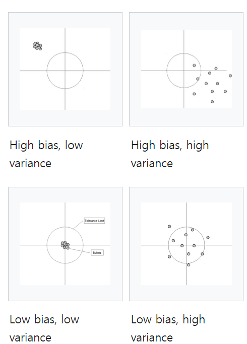
1. Underfitting: High Bias, Low Variance
   Underfitting occurs when a model is too simple to capture the underlying patterns in the data. This scenario is characterized by high bias and low variance, leading to poor performance on both training and test data. The model makes overly simplistic assumptions and fails to capture important features.

   Example: Using linear regression for a clearly non-linear relationship.

2. Overfitting: Low Bias, High Variance
   Overfitting happens when a model is too complex, memorizing the training data, including its noise. This results in low bias but high variance. The model performs excellently on training data but poorly on new, unseen data.

   Example: A decision tree with many levels that creates branches for almost every training example.

3. Ideal Scenario: Low Bias, Low Variance
   The goal is to achieve a model with both low bias and low variance, striking the right balance between complexity and generalization. This results in good performance across both training and test datasets.

   Example: A well-tuned random forest or a regularized regression model.

Calculating Bias and Variance

Understanding how to calculate bias and variance is crucial for diagnosing model performance and guiding improvement efforts. While the concepts are theoretical, there are practical ways to estimate them empirically.

Mathematical Formulas:

Let's define some terms:

• f(x): The true underlying function we're trying to approximate
• f̂(x): Our model's prediction
• E[f̂(x)]: The expected value of our model's prediction across different training sets

Bias is defined as the difference between the expected prediction of our model and the true value: Bias[f̂(x)] = E[f̂(x)] - f(x)

Variance is the variability of a model's predictions for a given data point: Variance[f̂(x)] = E[(f̂(x) - E[f̂(x)])²]

The total error can be decomposed as: Error = (Bias)² + Variance + Irreducible Error

In practice, we don't have access to the true function f(x) or multiple training sets to compute E[f̂(x)]. However, we can estimate bias and variance using techniques like bootstrapping or cross-validation.

Python Code Example:

Here's a simple example using sklearn to estimate bias and variance through cross-validation:

import numpy as np
from sklearn.model_selection import cross_val_predict
from sklearn.metrics import mean_squared_error

def bias_variance_decomp(model, X, y, cv=5):
    # Get cross-validated predictions
    y_pred = cross_val_predict(model, X, y, cv=cv)
    
    # Calculate MSE (total error)
    mse = mean_squared_error(y, y_pred)
    
    # Estimate bias
    bias = np.mean((y - y_pred)**2)
    
    # Estimate variance
    variance = np.var(y_pred)
    
    return mse, bias, variance

# Example usage:
from sklearn.datasets import make_regression
from sklearn.linear_model import LinearRegression

# Generate synthetic data
X, y = make_regression(n_samples=1000, n_features=10, noise=0.1)

# Create and fit model
model = LinearRegression()

# Compute bias and variance
mse, bias, variance = bias_variance_decomp(model, X, y)

print(f"MSE: {mse:.4f}")
print(f"Bias: {bias:.4f}")
print(f"Variance: {variance:.4f}")

This code provides estimates of bias and variance, but it's important to note that these are approximations. The true bias and variance would require knowledge of the underlying data distribution and the ability to sample multiple training sets.

In practice, rather than focusing on the exact numerical values of bias and variance, it's often more useful to:

1. Compare these metrics across different models
2. Track how they change as you modify your model or dataset
3. Use them in conjunction with other performance metrics and domain knowledge

By monitoring these estimates as you develop and refine your models, you can gain insights into whether your changes are reducing bias, variance, or both, guiding your efforts to improve overall model performance.

Strategies to Reduce Bias and Variance

Effectively managing the bias-variance tradeoff is key to developing high-performing machine learning models. Here are some strategies to reduce bias and variance, along with cross-validation approaches to help evaluate your efforts.

Techniques for Reducing High Bias:

1. Increase model complexity: Use more sophisticated models that can capture complex patterns in the data.

   • Example: Switch from linear regression to polynomial regression or decision trees.

2. Add more features: Include additional relevant features that might help explain the target variable.

   • Caution: Be mindful of the curse of dimensionality and potential overfitting.

3. Reduce regularization: If using regularization techniques, try reducing their strength to allow the model more flexibility.

   • Example: Decrease the lambda parameter in ridge or lasso regression.

4. Ensemble methods: Combine multiple high-bias models to create a more flexible ensemble.

   • Example: Use boosting algorithms like AdaBoost or Gradient Boosting.

5. Deep learning: For complex problems, consider using neural networks with multiple layers.

   • Note: This requires sufficient data and computational resources.

Methods for Reducing High Variance:

1. Increase training data: More data helps the model distinguish true patterns from noise.

   • Note: Ensure the new data is representative and high-quality.

2. Feature selection/reduction: Remove irrelevant features that might be causing the model to fit to noise.

   • Techniques: Use methods like PCA, Lasso, or domain knowledge-based selection.

3. Increase regularization: Apply or increase regularization to constrain the model's complexity.

   • Examples: L1/L2 regularization, dropout for neural networks.

4. Ensemble methods: Combine multiple high-variance models to create a more stable ensemble.

   • Example: Use bagging techniques like Random Forests.

5. Cross-validation: Use k-fold cross-validation to get a more robust estimate of model performance.

6. Simplify the model: Consider using a simpler model architecture that's less prone to overfitting.

   • Example: Reduce the depth of a decision tree or the number of layers in a neural network.

Cross-validation Approaches:

Cross-validation is crucial for assessing how well your model generalizes to unseen data. Here are some common approaches:

1. K-Fold Cross-Validation:

   • Split the data into K subsets
   • Train on K-1 subsets and validate on the remaining subset
   • Repeat K times, using each subset as the validation set once
   • Average the results for a robust performance estimate

2. Stratified K-Fold:

   • Similar to K-Fold, but ensures that the proportion of samples for each class is roughly the same in each fold
   • Particularly useful for imbalanced datasets

3. Leave-One-Out Cross-Validation (LOOCV):

   • Special case of K-Fold where K equals the number of samples
   • Computationally expensive but useful for small datasets

4. Time Series Cross-Validation:

   • For time-dependent data, use past observations to predict future observations
   • Ensures that you're not using future data to predict past events

Example Python code for K-Fold Cross-Validation:

from sklearn.model_selection import cross_val_score
from sklearn.linear_model import LinearRegression

# Assuming X and y are your features and target
model = LinearRegression()

# Perform 5-fold cross-validation
scores = cross_val_score(model, X, y, cv=5)

print(f"Cross-validation scores: {scores}")
print(f"Mean score: {scores.mean():.4f} (+/- {scores.std() * 2:.4f})")

By applying these strategies and using cross-validation to evaluate your models, you can work towards finding the optimal balance between bias and variance. Remember that the goal is not to eliminate bias and variance entirely (which is impossible), but to find the sweet spot that minimizes overall error and produces a model that generalizes well to new data.