Confidence Interval and IQR

Confidence Level

A confidence level is a measure of the reliability of a statistical estimate. It represents the probability that the true population parameter falls within a specified range (confidence interval) around the sample estimate. Common confidence levels include 90%, 95%, and 99%.

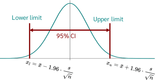
For example, a 95% confidence level means that if we were to repeat the sampling process many times, about 95% of the calculated confidence intervals would contain the true population parameter.

The formula for a confidence interval is:

$$\text{CI} = \bar{X} \pm (z \times \frac{s}{\sqrt{n}})$$

Where:

• $\bar{X}$ = sample mean
• $z$ = z-score corresponding to the desired confidence level
• $s$ = sample standard deviation
• $n$ = sample size

Confidence Intervals, Skewness, and Kurtosis

1. Confidence Intervals: A confidence interval is a range of values that is likely to contain the true population parameter with a certain level of confidence, typically 95%. It consists of a lower bound, a point estimate (usually the sample mean), and an upper bound. The width of the interval indicates the precision of the estimate, with narrower intervals suggesting more precise estimates.

Source : datatab

2. Skewness:

Source : Geeks for Geeks

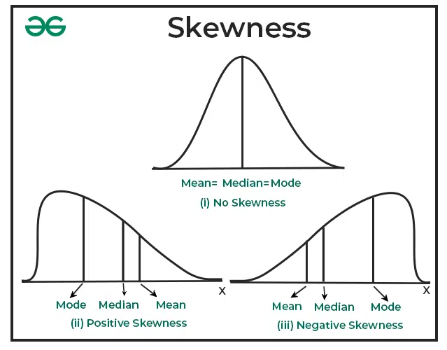
Skewness measures the asymmetry of a probability distribution. It can be:

• Zero skew (symmetric): The left and right sides of the distribution are mirror images.
• Positive skew (right-skewed): The tail of the distribution is longer on the right side.
• Negative skew (left-skewed): The tail of the distribution is longer on the left side.

Skewness affects the shape of the confidence interval and can influence the interpretation of statistical measures.

3. Kurtosis: Kurtosis is a measure of the "tailedness" of a probability distribution. It describes the shape of a distribution's tails in relation to its overall shape. Kurtosis is often misunderstood as a measure of peakedness, but it actually quantifies the presence of outliers or extreme values.

Types of Kurtosis:

Source : datakuity

a) Mesokurtic(중첨): This is the baseline kurtosis, typically associated with a normal distribution. It has a kurtosis value of 3 (or excess kurtosis of 0).

b) Leptokurtic(양의 첨도, 급첨): Distributions with positive excess kurtosis (>3) are leptokurtic. They have heavier tails and more extreme values than a normal distribution.

c) Platykurtic(음의 첨도, 완첨): Distributions with negative excess kurtosis (<3) are platykurtic. They have lighter tails and fewer extreme values than a normal distribution.

Importance of Kurtosis:

• In finance, kurtosis is used as a measure of financial risk. Higher kurtosis indicates a higher probability of extreme returns, both positive and negative.
• It helps in understanding the likelihood of outliers in a dataset.
• Kurtosis is crucial for assessing the appropriateness of statistical models and tests that assume normality.

Relationship between Confidence Intervals, Skewness, and Kurtosis:

1. These concepts collectively provide a comprehensive understanding of a distribution's shape and characteristics.
2. Skewness and kurtosis can affect the symmetry and width of confidence intervals.
3. In skewed or high-kurtosis distributions, traditional confidence intervals based on normal distribution assumptions may be less accurate.
4. For non-normal distributions (those with significant skewness or kurtosis), alternative methods like bootstrap confidence intervals might be more appropriate.

Standard Scalar (Standard Score or Z-score)

A standard scalar, often referred to as a z-score, is a measure of how many standard deviations an observation or data point is from the mean. It allows for comparison between different normal distributions and is calculated as:

$$z = \frac{(X - \mu)}{\sigma}$$

Where:

• $X$ = individual value
• $\mu$ = population mean
• $\sigma$ = population standard deviation

Z-scores are particularly useful in determining confidence intervals and hypothesis testing.

Interquartile Range (IQR)

The Interquartile Range (IQR) is a measure of statistical dispersion that represents the middle 50% of the data. It's calculated as:

$IQR = Q3 - Q1$

Where Q1 is the first quartile (25th percentile) and Q3 is the third quartile (75th percentile).

Visualization

Source : Saul McLeod, PhD

1. Box:

   • Bottom of the box: Q1 (First quartile, 25th percentile)
   • Top of the box: Q3 (Third quartile, 75th percentile)
   • Height of the box: IQR (Interquartile Range, Q3 - Q1)

2. Median line:

   • Horizontal line inside the box: Median (50th percentile)

3. Whiskers:

   • Lower whisker: Minimum value or Q1 - 1.5 * IQR, whichever is larger
   • Upper whisker: Maximum value or Q3 + 1.5 * IQR, whichever is smaller

4. Outliers:

   • Points beyond the whiskers: Values less than Q1 - 1.5 * IQR or greater than Q3 + 1.5 * IQR

This diagram, often called a box-and-whisker plot or boxplot, provides a visual summary of the data distribution. The box represents the middle 50% of the data, while the whiskers show the overall range of the data. The median line indicates the central tendency and helps in assessing the symmetry of the distribution.

Key points:

• The box contains 50% of the data.
• The distance between Q1 and Q3 (the IQR) is a measure of variability.
• The position of the median line relative to Q1 and Q3 indicates skewness.
• Whiskers and outliers provide information about the spread and potential extreme values in the dataset.

Related Concepts and Measures

1. T-score

A t-score is similar to a z-score but is used when the population standard deviation is unknown and the sample size is small (typically $n < 30$). T-scores are based on the t-distribution rather than the normal distribution.

2. Range

The range is defined as the difference between the maximum and minimum values in a dataset:

$Range = Max - Min$

3. Standard Deviation

The Standard Deviation measures the average distance between each data point and the mean. For a sample, it's calculated as:

$s = \sqrt{\frac{\sum_{i=1}^n (x_i - \bar{x})^2}{n - 1}}$

Where $x_i$ are individual values, $\bar{x}$ is the mean, and $n$ is the sample size.

4. Variance

Variance is the square of the standard deviation:

$s^2 = \frac{\sum_{i=1}^n (x_i - \bar{x})^2}{n - 1}$

5. Standard Error

The standard error (SE) is the standard deviation of the sampling distribution of a statistic. It's often used in calculating confidence intervals and is given by:

$$SE = \frac{s}{\sqrt{n}}$$

6. Margin of Error

The margin of error (ME) represents the range of values above and below the sample statistic in a confidence interval. It's calculated as:

$$ME = z \times SE$$

7. Effect Size (효과 크기)

Effect size is a standardized measure that quantifies the magnitude of the difference between groups or the strength of a relationship between variables.

Key features:

1. Ease of interpretation(해석의 용이성): Being standardized, it allows for comparison across different studies or scales.

2. Practical significance(실질적 중요성): Unlike statistical significance (p-value), it represents the actual magnitude of an effect.

3. Various measures(다양한 지표): Common indicators include Cohen's d, Pearson's r, and odds ratio.

4. Utility in meta-analysis(메타분석에서의 활용): Plays a crucial role in synthesizing results from multiple studies.

Cohen's general guidelines for interpreting effect sizes:

• Small: d = 0.2
• Medium: d = 0.5
• Large: d = 0.8

However, these interpretations can vary depending on the field and context.

Calculation example (Cohen's d):

$d = \frac{\bar{X}_1 - \bar{X}_2}{s_{\text{pooled}}}$

Where $\bar{X}_1$ and $\bar{X}_2$ are group means, and $s_{\text{pooled}}$ is the pooled standard deviation.

Odds Ratio (OR)

The Odds Ratio is a statistical measure that quantifies the strength of association between two events. It's widely used in epidemiology, medical research, and social sciences.

1. Definition: The Odds Ratio is the ratio of the odds of an event occurring in one group to the odds of it occurring in another group.

2. Calculation: $OR = \frac{Odds_1}{Odds_2} = \frac{p_1/(1-p_1)}{p_2/(1-p_2)}$ Where p1 and p2 are the probabilities of the event occurring in each group.

3. Interpretation:

   • OR = 1: No difference between the groups
   • OR > 1: The event is more likely to occur in group 1 compared to group 2
   • OR < 1: The event is less likely to occur in group 1 compared to group 2

4. Characteristics:

   • Range from 0 to infinity
   • Symmetrical distribution when log-transformed

5. Example Usage: In case-control studies, OR is often used to compare the likelihood of exposure in individuals with a disease (cases) to the likelihood of exposure in individuals without the disease (controls).

6. Advantages:

   • Relatively easy to interpret
   • Can be directly obtained from logistic regression
   • Useful in retrospective studies

7. Considerations:

   • When the event is rare, OR approximates the Relative Risk (RR)
   • For common events, OR may overestimate the RR

8. Practical Application: Let's consider a study examining the relationship between smoking and lung cancer:

   Group	Cancer	No Cancer	Total
   Smokers	60	140	200
   Non-smokers	30	170	200

   Odds of cancer in smokers: 60/140 = 0.429 Odds of cancer in non-smokers: 30/170 = 0.176

   OR = 0.429 / 0.176 = 2.44

   Interpretation: Smokers have 2.44 times higher odds of developing lung cancer compared to non-smokers.

9. Confidence Interval: It's important to calculate the confidence interval for the OR to assess its precision. The 95% CI for the log(OR) is typically calculated and then exponentiated:

   $95\% CI = e^{\ln(OR) \pm 1.96 \times SE(\ln(OR))}$

   Where SE is the standard error of the log odds ratio.

10. Relationship with Logistic Regression: In logistic regression, the exponential of the regression coefficient (e^β) for a predictor variable is the odds ratio for that predictor.

11. Limitations:

    • Can be misleading if misinterpreted as relative risk, especially for common outcomes
    • Sensitive to how data are organized in 2x2 tables

8. Statistical Power (검정력)

Power is the probability of correctly rejecting a false null hypothesis. In other words, it's the ability to detect an effect when it truly exists.

Key features:

1. Relationship with Type II error: Power = 1 - β (where β is the probability of Type II error)

2. Relationship with sample size: Power increases as sample size increases.

3. Relationship with effect size: Larger effect sizes lead to higher power.

4. Relationship with significance level: Increasing the significance level (α) increases power but also increases the probability of Type I error.

Generally, researchers aim for a power of 0.8 (80%) or higher.

Power can be calculated using this general formula:

$\text{Power} = 1 - \beta = P(|T| > t_{\alpha/2} | H_1 \text{ is true})$

Where T is the test statistic and $t_{\alpha/2}$ is the critical value.

Relationship between Effect Size and Power

1. Interdependence: Larger effect sizes result in higher power for the same sample size.

2. Research design: Both should be considered when determining appropriate sample sizes.

3. Result interpretation: When interpreting non-significant results, both effect size and power should be considered.

4. Practical importance: Effect size indicates the magnitude of the effect, while power represents the ability to detect that effect, making both crucial for assessing practical significance.

Practical Application

Consider a study comparing two teaching methods:

• Method A: Mean score = 75, SD = 10
• Method B: Mean score = 80, SD = 10
• Sample size: 50 students per group

1. Calculate Effect Size (Cohen's d):

   $d = \frac{80 - 75}{10} = 0.5$

   This indicates a medium effect size.

2. Calculate Power: Assuming α = 0.05, we can use statistical software or power tables to find that the power is approximately 0.70 or 70%.

3. Interpretation: The effect size of 0.5 suggests a moderate practical difference between the methods. However, the power of 70% indicates a 30% chance of failing to detect this difference if it truly exists. Researchers might consider increasing the sample size to improve power.

9. P-value

The p-value indicates the probability of obtaining test results at least as extreme as observed results, assuming that the null hypothesis is correct.

10. Mean Absolute Deviation (MAD)

The MAD is the average of the absolute deviations from the mean:

$MAD = \frac{\sum_{i=1}^n |x_i - \bar{x}|}{n}$

11. Coefficient of Variation (CV)

The CV is the ratio of the standard deviation to the mean, often expressed as a percentage:

$CV = \frac{s}{\bar{x}} \times 100\%$

12. Quartile Deviation (Semi-Interquartile Range)

The Quartile Deviation is half the IQR:

$QD = \frac{Q3 - Q1}{2}$

13. Percentile Range

Similar to IQR, but using different percentiles. For example, the 10-90 percentile range:

$PR_{10-90} = P_{90} - P_{10}$

Where $P_{90}$ is the 90th percentile and $P_{10}$ is the 10th percentile.

Comparison of Dispersion Measures

Measure	Advantages	Disadvantages
IQR	Robust to outliers, good for skewed data	Ignores 50% of data
Range	Simple to calculate and understand	Highly sensitive to outliers
Standard Deviation	Uses all data points, widely used	Sensitive to outliers
Variance	Useful in many statistical analyses	Not in same units as data
MAD	Robust to outliers	Less commonly used
CV	Allows comparison between datasets with different units	Not suitable for data with mean near zero
Quartile Deviation	Robust to outliers, easy to interpret	Ignores 50% of data
Percentile Range	Flexible, can focus on different parts of distribution	May ignore extreme values

Conclusion

These statistical concepts and measures are interconnected and provide various ways to analyze and interpret data. The choice of which measure to use depends on the nature of your data, the specific questions you're trying to answer, and the assumptions you can make about your data's distribution.

Understanding these concepts is crucial for interpreting statistical results, designing experiments, and making data-driven decisions. They provide a framework for quantifying uncertainty, measuring dispersion, and making inferences about populations based on sample data.

When working with real-world data, it's often beneficial to use multiple measures to gain a comprehensive understanding of your dataset's characteristics. This approach allows you to balance the strengths and weaknesses of different statistical measures and make more informed decisions based on your analysis.