CNN (Convolutional Neural Network) Explanation Part. 2

Part 2. CNN's Major Architectures and Applications

1. Introduction to Famous CNN Architectures

Convolutional Neural Network (CNN) architectures have led revolutionary advancements in the field of computer vision. Let's examine the development process of major CNN architectures. I will show you again my ugly image of CNN architetures. :)

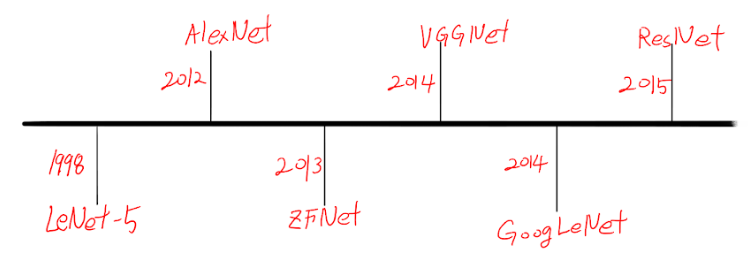
LeNet-5

LeNet-5, developed in 1998 by Yann LeCun, Léon Bottou, Yoshua Bengio, and Patrick Haffner, is an early CNN architecture. It was primarily designed for recognizing handwritten digits on checks and postal codes. The structure of LeNet-5 is as follows:

1. Input layer: 32x32 pixel grayscale image
2. C1: Convolutional layer with 6 feature maps using 5x5 kernels
3. S2: Average pooling layer with 2x2 kernels
4. C3: Convolutional layer with 16 feature maps using 5x5 kernels
5. S4: Average pooling layer with 2x2 kernels
6. C5: Convolutional layer with 120 feature maps using 5x5 kernels
7. F6: Fully connected layer with 84 units
8. Output layer: Fully connected layer with 10 units (for classifying digits 0-9)

LeNet-5 has about 60,000 trainable parameters and uses the tanh activation function. This model is significant as it first introduced the basic structure of modern CNNs: a combination of convolutional layers, pooling layers, and fully connected layers. It also introduced the concept of stacking layers to learn complex features.

Please visit here for more.

AlexNet

AlexNet, developed in 2012 by Alex Krizhevsky, Ilya Sutskever, and Geoffrey Hinton, won the ImageNet Large Scale Visual Recognition Challenge (ILSVRC) 2012. The structure of AlexNet is as follows:

1. Input layer: 227x227x3 RGB image
2. Conv1: 96 filters of size 11x11, stride 4, ReLU activation
3. MaxPool1: 3x3 kernel, stride 2
4. Conv2: 256 filters of size 5x5, padding 2, ReLU activation
5. MaxPool2: 3x3 kernel, stride 2
6. Conv3: 384 filters of size 3x3, padding 1, ReLU activation
7. Conv4: 384 filters of size 3x3, padding 1, ReLU activation
8. Conv5: 256 filters of size 3x3, padding 1, ReLU activation
9. MaxPool3: 3x3 kernel, stride 2
10. FC6: 4096 units, ReLU activation, dropout
11. FC7: 4096 units, ReLU activation, dropout
12. FC8: 1000 units (output layer)

AlexNet has about 60 million parameters and introduced several innovative features:

1. ReLU activation function: Used ReLU instead of tanh or sigmoid, greatly improving learning speed.
2. Dropout: Applied dropout to fully connected layers to prevent overfitting.
3. Data augmentation: Used techniques like image rotation, flipping, and color changes to augment training data.
4. GPU usage: Used two GPUs in parallel to significantly improve training speed.

AlexNet achieved a top-5 error rate of 15.3% in ILSVRC 2012, significantly outperforming the second-place entry (26.2%). This demonstrated the superiority of deep learning and sparked a boom in deep learning research in the computer vision field.

Please visit here for more.

VGGNet

VGGNet, developed in 2014 by the Visual Geometry Group at Oxford University (Karen Simonyan, Andrew Zisserman), is characterized by its very uniform architecture. There are two versions, VGG16 and VGG19, with VGG16's structure as follows:

1. Input layer: 224x224x3 RGB image
2. Two 3x3 convolutional layers (64 channels) + MaxPooling
3. Two 3x3 convolutional layers (128 channels) + MaxPooling
4. Three 3x3 convolutional layers (256 channels) + MaxPooling
5. Three 3x3 convolutional layers (512 channels) + MaxPooling
6. Three 3x3 convolutional layers (512 channels) + MaxPooling
7. Three fully connected layers (4096, 4096, 1000 units)

VGGNet's main innovations are:

1. Small filter size: Used only 3x3 filters in all convolutional layers, allowing for a wider receptive field with fewer parameters.
2. Deep network: VGG16 has 16 layers and VGG19 has 19 layers, which were very deep networks at the time.
3. Uniform structure: All convolutional layers use the same padding and stride, resulting in a very simple structure.

While VGGNet placed second in ILSVRC 2014 behind GoogLeNet, its simple and uniform structure made it widely used by many researchers. However, with about 138 million parameters, it has the drawback of high memory usage and long training times.

Please visit here for more.

GoogLeNet

Source : Geeks for Geeks

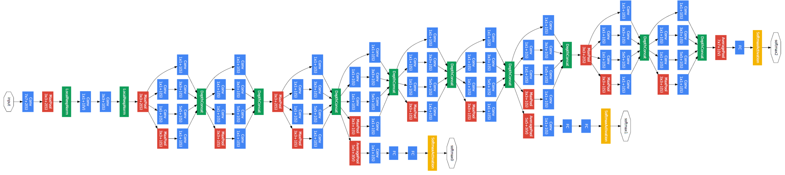
GoogLeNet, developed by Google in 2014, won the ILSVRC 2014 competition. Its main features are:

1. Inception module: The core component of GoogLeNet, performing convolutions with filters of various sizes and pooling operations in parallel.
2. 1x1 convolutions: Used for dimension reduction, reducing computation and increasing network depth.
3. Deep structure: Composed of 22 layers, making it one of the deepest networks at the time.
4. Auxiliary classifiers: Used additional classifiers in intermediate layers to mitigate the vanishing gradient problem.
5. Efficient parameter use: Achieved higher performance with 12 times fewer parameters than AlexNet.

ResNet

Please visit wiki for more.

ResNet (Residual Network), developed by Microsoft Research in 2015, won ILSVRC 2015. Its main features are:

1. Residual Learning: Uses skip connections that directly add the input of a layer to its output.
2. Very deep structure: Various versions exist, such as ResNet-50, ResNet-101, ResNet-152, with networks of over 1000 layers possible to train.
3. Solving the vanishing gradient problem: Skip connections allow gradients to be directly passed to previous layers, enabling the training of very deep networks.
4. Bottleneck Architecture: Uses 1x1 convolutions to reduce and increase dimensions, improving computational efficiency.
5. Batch Normalization: Applied after each convolutional layer to increase learning stability.

ResNet presented a method to effectively train even deeper structures than GoogLeNet and has since been used as a base model in many computer vision tasks.

2. Recent CNN Architectures

EfficientNet

Paper : EfficientNet: Rethinking Model Scaling for Convolutional Neural Networks

EfficientNet, introduced by Google researchers in 2019, represents a significant advancement in CNN architecture design. Its key innovation is the use of compound scaling to systematically scale network depth, width, and resolution.

Key features:

1. Compound Scaling: Uniformly scales network width, depth, and resolution using a compound coefficient.
2. Mobile Inverted Bottleneck Convolution (MBConv): Uses depthwise separable convolutions for efficiency.
3. Squeeze-and-Excitation blocks: Improves channel interdependencies.

Performance: EfficientNet-B7 achieved state-of-the-art 84.4% top-1 accuracy on ImageNet while being 8.4 times smaller and 6.1 times faster than the previous best model.

Vision Transformers (ViT)

Paper : An Image is Worth 16x16 Words: Transformers for Image Recognition at Scale

Vision Transformers, introduced by Google researchers in 2020, apply the transformer architecture, originally designed for natural language processing, to image recognition tasks.

Key features:

1. Patch-based input: Divides images into fixed-size patches.
2. Positional embeddings: Maintains spatial information.
3. Self-attention mechanism: Allows for global context understanding.

Performance: When pre-trained on large datasets, ViT outperforms ResNet models of similar size, achieving 88.55% top-1 accuracy on ImageNet.

3. Performance Comparisons

Here's a comparison of top-1 accuracy on ImageNet for various architectures:

Model	Top-1 Accuracy	Parameters	Year
AlexNet	63.3%	60M	2012
VGG16	71.5%	138M	2014
GoogLeNet	69.8%	6.8M	2014
ResNet-50	76.0%	25.6M	2015
ResNet-152	78.3%	60.2M	2015
DenseNet-201	77.4%	20M	2017
EfficientNet-B7	84.4%	66M	2019
ViT-L/16	85.3%	307M	2020

This comparison shows the trend of increasing accuracy over time, often with a reduction in parameter count, demonstrating the efficiency improvements in newer architectures.

4. Major Application Areas of CNNs

Image Classification

Image classification is the most basic and well-known application area of CNNs.

Real-world applications:

• Medical image diagnosis: CNNs are used to analyze medical images such as X-rays, MRIs, and CT scans to diagnose various diseases including cancer, pneumonia, and fractures. For example, a research team at Stanford University developed a CNN model called CheXNet that successfully diagnoses pneumonia from chest X-ray images.
• Autonomous vehicles: Companies like Tesla and Waymo use CNNs to recognize and classify objects around the vehicle (pedestrians, other vehicles, traffic signs, etc.).
• Social media image tagging: Platforms like Facebook and Instagram use CNNs to automatically recognize the content of user-uploaded images and generate tags.

Object Detection

Object detection involves locating and classifying specific objects within an image.

Real-world applications:

• Security systems: Real-time detection of suspicious objects or behaviors in CCTV footage at airports, shopping malls, etc. For example, companies like Avigilon integrate CNN-based object detection technology into their security camera systems.
• Manufacturing quality control: Automatic detection of product defects on production lines. Companies like Cognex provide CNN-based machine vision systems to manufacturers to automate quality control processes.
• Retail inventory management: Unmanned stores like Amazon Go use CNN-based object detection technology to automatically recognize and charge for products selected by customers.

Segmentation

Segmentation involves classifying each pixel in an image into a specific class.

Real-world applications:

• Medical image analysis: Used to find precise boundaries of tumors in brain MRI images or segment blood vessels in retinal images. For example, DeepMind's research team developed a system to diagnose eye diseases using a CNN-based segmentation model.
• Autonomous vehicles: Accurately distinguishing roads, sidewalks, lanes, etc. to plan safe driving routes. Companies like Mobileye apply CNN-based segmentation technology to autonomous driving systems.
• Satellite image analysis: Automatically classifying areas of farmland, cities, forests, etc. for environmental monitoring or urban planning. Companies like Planet Labs provide segmentation analysis services for satellite images using CNNs.

Face Recognition

CNNs have also achieved great success in the field of face recognition.

Real-world applications:

• Smartphone unlocking: CNN-based face recognition technology is used in features like Apple's Face ID and Android's face recognition.
• Airport security systems: Many countries use CNN-based face recognition technology to automate passport verification and security screening processes.
• Social media tagging: Facebook uses a CNN-based face recognition system called DeepFace to automatically tag users in photos.

CNNs are being used in various industries and their range of applications continues to expand through ongoing research and development.

5. Latest Advancements in CNN Applications

1. Medical Imaging: CNNs are being used for early detection of diseases like diabetic retinopathy and skin cancer. For instance, a CNN-based system developed by Google Health achieved expert-level accuracy in detecting breast cancer from mammograms.

2. Autonomous Driving: Advanced CNN architectures are being used for real-time object detection, semantic segmentation, and depth estimation in self-driving cars. Companies like Tesla are using CNNs for their Full Self-Driving (FSD) technology.

3. Deepfake Detection: CNNs are being employed to detect manipulated images and videos, which is crucial for combating misinformation.

4. Super-Resolution: CNN-based models like ESRGAN (Enhanced Super-Resolution Generative Adversarial Network) can upscale low-resolution images with impressive detail.

5. Video Understanding: Models like SlowFast networks use CNNs to analyze spatial and temporal information in videos for action recognition and video classification.

6. Visualization and Interpretation of CNNs

Filter Visualization

Filter visualization is a technique for visualizing the convolutional filters in each layer of a CNN.

1. Direct weight visualization:

   • Directly convert the weights of each filter into an image for visualization.
   • Filters in early layers typically detect low-level features such as edges, colors, and textures.
   • Filters in deeper layers detect more complex and abstract patterns.

2. Activation maximization:

   • Generate input images that maximize the activation of a specific filter.
   • Start from random noise and optimize the image to maximize the activation of the target filter.
   • This allows for visual confirmation of what patterns each filter responds to.

Activation Map Visualization

Activation maps (or feature maps) are intermediate representations generated when an input image passes through each convolutional layer.

1. Intermediate layer activation maps:

   • Visualize the activation maps of each layer as heatmaps.
   • This shows which parts of the image the network focuses on.

2. Class Activation Mapping (CAM):

   • Applicable to CNNs using a Global Average Pooling layer.
   • Combines feature maps from the last convolutional layer with class-specific weights to generate class-specific activation maps.
   • Shows which regions of the image the model focused on when predicting a specific class.

Grad-CAM

Grad-CAM (Gradient-weighted Class Activation Mapping) is an improved technique over CAM that can be applied to all CNN architectures.

1. Working principle:

   • Calculate gradients for the target class.
   • Use these gradients as weights for the activation maps of the last convolutional layer.
   • Combine the weighted activation maps to generate the final heatmap.

2. Advantages:

   • Can be applied without modifying the model architecture.
   • Can explain the model's decisions for each class.

Saliency Maps

Saliency Maps visualize the influence of each pixel in the input image on the final prediction.

1. Calculation method:

   • Calculate the gradient of the input image with respect to the score of the target class.
   • Take the absolute value of the gradient to represent the importance of each pixel.

2. Interpretation:

   • Bright areas indicate pixels that have a large influence on the prediction.
   • Dark areas indicate pixels that have little influence on the prediction.

Guided Backpropagation

Guided Backpropagation is an improved technique over Saliency Maps.

1. Features:

   • Only propagates positive gradients during backpropagation.
   • Effective in networks using ReLU activation functions.

2. Results:

   • Can visualize features in the input space more clearly.
   • Emphasizes the contours and main features of objects.

Integrated Gradients

Integrated Gradients calculates the importance of each pixel by integrating the gradient path from a baseline image (usually a black image) to the input image.

1. Advantages:

   • Provides results with less noise and easier interpretation than Saliency Maps.
   • Provides more accurate attribution for the model's predictions.

2. Calculation process:

   • Generate several intermediate images from the baseline image to the input image.
   • Calculate gradients for each intermediate image and integrate them.

These visualization and interpretation techniques greatly help in understanding and explaining the decision-making process of CNN models. They allow for the discovery and improvement of model biases or errors and play an important role in the field of Explainable AI.

Source : Gao Hongnan

7. Latest Advancements in CNN Interpretation Techniques

1. SHAP (SHapley Additive exPlanations): This technique uses game theory concepts to explain the output of any machine learning model, including CNNs.

2. Layer-wise Relevance Propagation (LRP): LRP provides pixel-wise explanations for CNN decisions by redistributing the prediction score back to the input pixels.

3. Concept Activation Vectors (CAVs): This technique allows for testing of high-level concepts within CNN layers, providing more human-interpretable explanations.

4. Adversarial Examples: While primarily a security concern, adversarial examples also serve as a tool for understanding CNN vulnerabilities and improving interpretability.

5. Neural Style Transfer Improvements: Advanced techniques in style transfer, such as adaptive instance normalization, provide insights into how CNNs separate and recombine content and style information.

These advancements demonstrate the ongoing evolution of CNN architectures, their expanding applications, and the growing focus on making these powerful models more interpretable and trustworthy. As CNNs continue to develop, we can expect further improvements in efficiency, accuracy, and applicability across various domains.

8. Transfer Learning and Fine-tuning

Transfer Learning

Transfer learning is a technique that applies knowledge from a pre-trained model on a large dataset to a new task. It is particularly useful in CNNs.

Main advantages of transfer learning:

1. Reduced training time: Models can be trained much faster than learning from scratch.
2. Good performance with less data: Good performance can be achieved even with limited data for the new task.
3. Improved generalization: Using a pre-trained model that has learned various features can lead to good generalization performance on new tasks.

Main methods of transfer learning:

1. Using as a feature extractor: Fix the convolutional layers of the pre-trained model and only replace and train the last fully connected layer for the new task.
2. Fine-tuning: Adjust the weights of some or all layers of the pre-trained model for the new task.

Fine-tuning

Fine-tuning is the process of adapting a pre-trained model to better suit a new task.

Main techniques of fine-tuning:

1. Learning rate adjustment: Apply a low learning rate to pre-trained layers and a high learning rate to newly added layers.
2. Gradual unfreezing: Initially train only the last layer, then gradually include previous layers in the training.
3. Discriminative learning rates: Apply different learning rates to different parts of the network.

Fine-tuning process:

1. Select a pre-trained model: Choose a model trained on a domain similar to the target task.
2. Modify model structure: Modify the output layer to fit the new task.
3. Freeze layers: Freeze initial layers so their weights are not updated.
4. Train new layers: Train newly added layers with a high learning rate.
5. Fine-tune: Gradually unfreeze frozen layers and fine-tune the entire network with a low learning rate.

Transfer learning and fine-tuning are particularly useful techniques in situations where data is limited or computational resources are scarce. These methods allow for high-performance models to be obtained with small amounts of data and significantly reduce training time.

Source : Geeks for Geeks

In conclusion, the major architectures of CNNs, their application areas, transfer learning and fine-tuning techniques, and visualization and interpretation methods are all closely related. They evolve together, driving innovation in the field of computer vision. The development of CNN architectures creates more accurate and efficient models, leading to performance improvements in various application areas. Transfer learning and fine-tuning allow these high-performance models to be utilized in more situations, while visualization and interpretation techniques increase the reliability of models and enable continuous improvement.

In the future, CNN technology will continue to evolve, enabling the performance of more complex visual tasks. At the same time, research on model efficiency, interpretability, and ethical use will also progress. Through this, CNNs will become not just a technical tool, but a powerful tool that complements and extends human visual cognitive abilities.