CNN (Convolutional Neural Network) Explanation Part. 1

Part 1: CNN Basics and Structure

1. Introduction to CNN

Convolutional Neural Networks (CNNs) have revolutionized the field of machine learning, particularly in the domain of computer vision. To truly appreciate the power and significance of CNNs, it's essential to first understand the broader context of machine learning and deep learning.

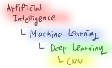
Machine learning is a subset of artificial intelligence that focuses on creating algorithms that can learn from and make predictions or decisions based on data. The key distinction of machine learning from traditional programming is its ability to improve its performance on a specific task through experience, without being explicitly programmed for every possible scenario.

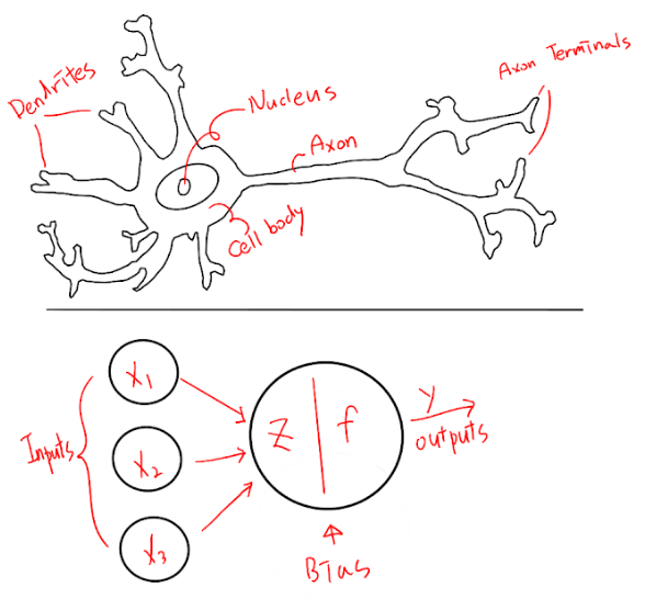
Within the realm of machine learning, deep learning has emerged as a particularly powerful approach. Deep learning uses artificial neural networks with multiple layers to model complex patterns in data. These neural networks are inspired by the structure and function of the human brain, consisting of interconnected nodes (neurons) that process and transmit information.

CNNs are a specialized type of neural network designed primarily for processing grid-like data, such as images. The key innovation of CNNs lies in their ability to automatically and adaptively learn spatial hierarchies of features from input data. This makes them incredibly effective for tasks involving image recognition, object detection, and even natural language processing.

The history of CNNs is a fascinating journey that spans several decades:

1. 1980s: Kunihiko Fukushima developed the Neocognitron, a hierarchical multi-layered artificial neural network. This was one of the first neural networks that incorporated the concepts of local receptive fields, shared weights, and hierarchical organization of cells, which are fundamental to modern CNNs.

2. 1989: Yann LeCun and his colleagues applied the backpropagation algorithm to a deep neural network for the purpose of recognizing handwritten digits. This work laid the foundation for modern CNNs.

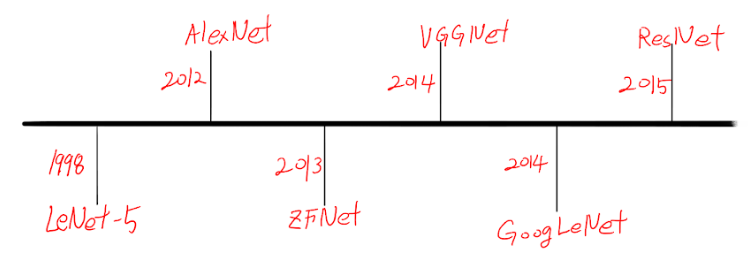
3. 1998: LeCun et al. introduced LeNet-5, the first modern CNN architecture. LeNet-5 was used for digit recognition and demonstrated the effectiveness of CNNs for handwritten character recognition.

4. 2012: The true potential of CNNs was realized when Alex Krizhevsky, Ilya Sutskever, and Geoffrey Hinton won the ImageNet Large Scale Visual Recognition Challenge with their AlexNet architecture. This breakthrough demonstrated the power of deep CNNs and sparked a revolution in computer vision and deep learning.

CNNs have several key characteristics that make them particularly effective for image processing tasks:

1. Local connectivity: Unlike fully connected networks where each neuron is connected to every neuron in the adjacent layers, CNNs exploit spatially local correlation by enforcing a local connectivity pattern between neurons of adjacent layers. This means that each neuron is only connected to a small region of the input volume. This approach significantly reduces the number of parameters in the network.

2. Shared weights: In CNNs, the same filter (weight matrix) is used for each pixel in the layer, significantly reducing the number of parameters that need to be learned. This property is based on the assumption that if a feature is useful to compute at some spatial position, it should also be useful to compute at other positions.

3. Pooling: CNNs typically use pooling layers to reduce the spatial dimensions of the representation. This makes the network less sensitive to small translations in the input, a property known as translation invariance.

4. Hierarchy of features: Through multiple layers, CNNs can learn hierarchical features. Early layers might learn to detect edges and simple shapes, while deeper layers can combine these to recognize more complex patterns and eventually entire objects or scenes.

Source : Chandra P.

These characteristics allow CNNs to efficiently process high-dimensional data like images while requiring fewer parameters than traditional fully connected neural networks. As a result, CNNs have become the go-to architecture for a wide range of computer vision tasks, including image classification, object detection, segmentation, and face recognition.

The impact of CNNs extends beyond just computer vision. Their ability to automatically learn hierarchical features has inspired developments in other areas of machine learning and artificial intelligence. For instance, CNNs have been adapted for use in natural language processing tasks, speech recognition, and even in analyzing time series data.

As we delve deeper into the structure and workings of CNNs in the following sections, keep in mind that we're exploring a technology that has not only transformed the field of computer vision but has also played a crucial role in the broader AI revolution we're experiencing today.

2. Basic Structure of CNNs

The architecture of a Convolutional Neural Network (CNN) is meticulously designed to take advantage of the 2D structure of input data, such as images. Understanding this architecture is crucial for grasping how CNNs achieve their remarkable performance in various tasks. Let's explore each component of a typical CNN in detail:

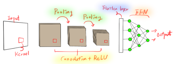
1. Input Layer: The input layer in a CNN is where the raw pixel values of the image are fed into the network. For a color image, this layer typically has three channels (Red, Green, and Blue), while for a grayscale image, it has a single channel. The dimensions of this layer correspond to the width, height, and depth (number of channels) of the input image.

For instance, a typical input for a CNN might be a 224x224 pixel color image, which would be represented as a 224x224x3 volume in the input layer.

2. Convolutional Layer: The convolutional layer is the core building block of a CNN. It performs a convolution operation, where a small window (kernel or filter) slides over the input data, performing element-wise multiplication and then summing to produce a single value in the output feature map.

Source : Glass Box

Key aspects of the convolutional layer include:

• Filters: Each filter is a set of learnable weights that detects specific features. A typical filter might be 3x3 or 5x5 in size. The network learns these filters during training to detect features that are most relevant to the task at hand.

• Stride: The step size of the filter as it slides across the input. A stride of 1 means the filter moves one pixel at a time, while a larger stride (e.g., 2 or 3) means the filter skips pixels, resulting in smaller output dimensions.

• Padding: Adding extra pixels around the input to control the output size. "Valid" padding means no padding is added, while "same" padding adds enough padding to ensure the output has the same spatial dimensions as the input.

The output of a convolutional layer is a set of feature maps, each representing the response of a particular filter at every spatial position in the input.

3. Activation Function: After each convolution operation, an activation function is applied to introduce non-linearity into the model. Non-linearity is crucial because it allows the network to learn complex patterns that a purely linear model could not capture.

The most common activation function used in CNNs is the Rectified Linear Unit (ReLU), which outputs the input directly if it is positive, or zero otherwise. Mathematically, it's expressed as f(x) = max(0, x).

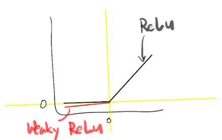
Other activation functions that might be used include:

• Leaky ReLU: Similar to ReLU, but allows a small, non-zero gradient when the input is negative.
• ELU (Exponential Linear Unit): Smoother than ReLU and can produce negative outputs.
• SELU (Scaled Exponential Linear Unit): Self-normalizing variant that can help with training very deep networks.

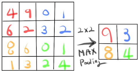
4. Pooling Layer: Pooling layers are periodically inserted between successive convolutional layers. Their function is to progressively reduce the spatial size of the representation, which helps to:

• Reduce the number of parameters and computation in the network
• Control overfitting
• Make the network invariant to small translations in the input

The most common pooling operation is max pooling, which outputs the maximum value within a rectangular neighborhood. For instance, a 2x2 max pooling layer with a stride of 2 will downsample the input by half in both spatial dimensions.

Other types of pooling include:

• Average pooling: Takes the average value in the pooling window
• Global pooling: Reduces each feature map to a single value, often used at the end of the network

5. Fully Connected Layer: After several convolutional and pooling layers, the high-level reasoning in the neural network is done via fully connected layers. Neurons in these layers have connections to all activations in the previous layer, as in regular neural networks.

The transition from convolutional layers to fully connected layers is typically done by flattening the output of the last convolutional layer into a 1D vector.

6. Output Layer: The output layer in a CNN is responsible for producing the final prediction. The nature of this layer depends on the specific task:

• For classification tasks, it often uses a softmax activation function to produce a probability distribution over the possible classes.
• For regression tasks, it might use a linear activation.
• For multi-label classification, it might use sigmoid activations for each output neuron.

The power of CNNs comes from their ability to learn hierarchical features. The early layers learn to detect low-level features like edges and textures, while deeper layers combine these to detect higher-level features and eventually entire objects. This hierarchical learning is what makes CNNs so effective at image recognition tasks.

Understanding this basic structure is crucial for designing effective CNN architectures. In practice, modern CNN architectures often incorporate additional elements like skip connections, inception modules, or attention mechanisms to further enhance their capabilities. As we progress through this series, we'll explore some of these advanced concepts and how they build upon this fundamental structure.

3. Key Concepts in CNNs

To truly grasp the power and effectiveness of Convolutional Neural Networks (CNNs), it's essential to understand several key concepts that underpin their operation. These concepts not only explain how CNNs work but also provide insights into why they are so effective for tasks involving grid-like data, particularly images. Let's delve deep into these crucial concepts:

1. Filters and Feature Maps:

Filters, also known as kernels, are the core components of CNNs. A filter is a small matrix of weights that slides over the input data, performing element-wise multiplication and summation to create a feature map. Each filter is designed to detect a specific pattern or feature in the input.

Source : Debugger Cafe

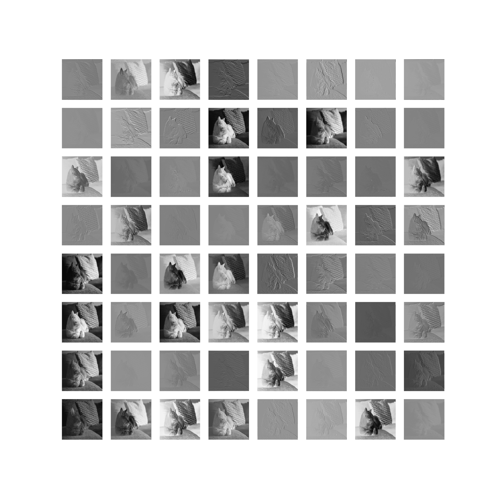
Feature maps are the outputs produced by applying a filter to an input. They represent the presence and location of specific features in the input. As the network deepens, feature maps become more abstract, representing higher-level concepts.

The process of learning in CNNs involves adjusting the weights of these filters to detect the most relevant features for the task at hand. This is done through backpropagation and gradient descent, which we'll discuss in more detail in the next section.

Importance of Filters and Feature Maps:

• They allow the network to learn spatial hierarchies of features.
• Different filters can specialize in detecting different types of features (e.g., edges, textures, shapes).
• The combination of multiple filters allows the network to capture a rich representation of the input.

2. Stride and Padding:

Stride refers to the step size of the filter as it slides across the input. A stride of 1 means the filter moves one pixel at a time, while a larger stride (e.g., 2 or 3) means the filter skips pixels, resulting in smaller output dimensions.

Source : Mallahyari Github

Padding involves adding extra pixels around the edges of the input. This is typically done to control the spatial size of the output volumes. Two common types of padding are:

• Valid padding: No padding is added, and the spatial dimensions are reduced.
• Same padding: Padding is added to ensure the output has the same spatial dimensions as the input.

Importance of Stride and Padding:

• They allow control over the spatial dimensions of the output feature maps.
• Proper use can help preserve information at the borders of the input.
• They can be used to reduce computational complexity by downsampling the input.

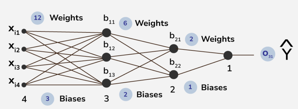
3. Parameter Sharing:

Parameter sharing is a key principle in CNNs that significantly reduces the number of parameters in the model. In a convolutional layer, the same filter is applied to every position of the input. This means that the weights are shared across the entire input, allowing the network to detect a feature regardless of its position in the image.

This concept is based on the assumption that if a feature is useful to compute at some spatial position, it should also be useful to compute at other positions. Parameter sharing not only reduces the number of parameters but also makes CNNs translation invariant, meaning they can detect features regardless of their location in the image.

Importance of Parameter Sharing:

• Drastically reduces the number of parameters in the model, preventing overfitting.
• Enables translation invariance, a crucial property for many computer vision tasks.
• Allows the network to generalize well to inputs of different sizes.

4. Receptive Field:

The receptive field refers to the region in the input space that a particular CNN feature is looking at. As we go deeper into the network, the receptive field of a unit becomes larger. This allows deeper layers to capture more complex and abstract features by combining information from a larger area of the original input.

Source : Lukas Fiederer

Understanding the receptive field is crucial for designing effective CNN architectures. It helps in determining the size of filters and the depth of the network required to capture features at different scales.

Importance of Receptive Field:

• Determines the scale of features that can be detected at each layer.
• Guides the design of network architecture for specific tasks.
• Helps in understanding the network's ability to capture context and global information.

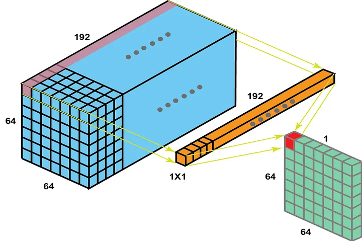
5. 1x1 Convolutions:

1x1 convolutions, also known as pointwise convolutions, are a special type of convolution where the filter size is 1x1. Despite their simplicity, they serve several important purposes:

• Dimensionality reduction: They can be used to reduce the number of channels in the input.
• Adding non-linearity: When followed by an activation function, they introduce additional non-linearity into the network.
• Cross-channel parametric pooling: They allow the network to create linear combinations of channels, enabling it to learn cross-channel correlations.

Source : Raj Sakthi

Importance of 1x1 Convolutions:

• Enable efficient network architectures by controlling the number of channels.
• Allow for more complex functions to be learned by increasing network depth without significantly increasing computational cost.
• Play a crucial role in modern architectures like Inception and ResNet.

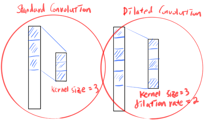
6. Dilated Convolutions:

Dilated (or atrous) convolutions introduce "holes" in the filters, effectively increasing the receptive field without increasing the number of parameters. This is particularly useful in tasks that require capturing long-range dependencies, such as semantic segmentation.

Importance of Dilated Convolutions:

• Allow for larger receptive fields without increasing the number of parameters or the amount of computation.
• Particularly useful in dense prediction tasks like semantic segmentation.
• Enable multi-scale feature extraction without the need for downsampling and upsampling operations.

Understanding these key concepts provides deeper insights into how CNNs process and learn from data. These principles guide the design and optimization of CNN architectures for various tasks. As we continue to explore CNNs, we'll see how these concepts are applied in practice and how they contribute to the remarkable performance of these networks in a wide range of applications.

In the next section, we'll delve into the learning process of CNNs, exploring how these networks are trained to perform their impressive feats of perception and recognition.

4. Learning Process in CNNs

The learning process in Convolutional Neural Networks (CNNs) is a sophisticated interplay of forward propagation, backpropagation, loss calculation, and optimization. Understanding this process is crucial for effectively training and fine-tuning CNN models. Let's break down the key components of the CNN learning process and explore each in detail:

1. Forward Propagation:

Forward propagation is the process of passing input data through the network to generate predictions. In a CNN, this involves the following steps:

a) Input layer: The raw image data is fed into the network. b) Convolutional layers: Filters are applied to the input, creating feature maps. c) Activation functions: Non-linearity is introduced, typically using ReLU. d) Pooling layers: The spatial dimensions are reduced. e) Fully connected layers: High-level reasoning is performed. f) Output layer: Final predictions are generated.

Source : Geeks for Geeks

During forward propagation, each layer performs its specific operation and passes the result to the next layer. The output of the final layer is the network's prediction.

2. Loss Function:

After forward propagation, the network's predictions are compared to the true labels using a loss function. The choice of loss function depends on the specific task. Common loss functions include:

• Cross-entropy loss: Used for classification tasks. It measures the dissimilarity between the predicted probability distribution and the true distribution.
• Mean Squared Error (MSE): Often used for regression tasks. It calculates the average squared difference between predicted and actual values.
• Focal loss: Useful for dealing with class imbalance by down-weighting the loss contributed by easy examples.

The loss function quantifies how well the network's predictions match the true labels. The goal of training is to minimize this loss.

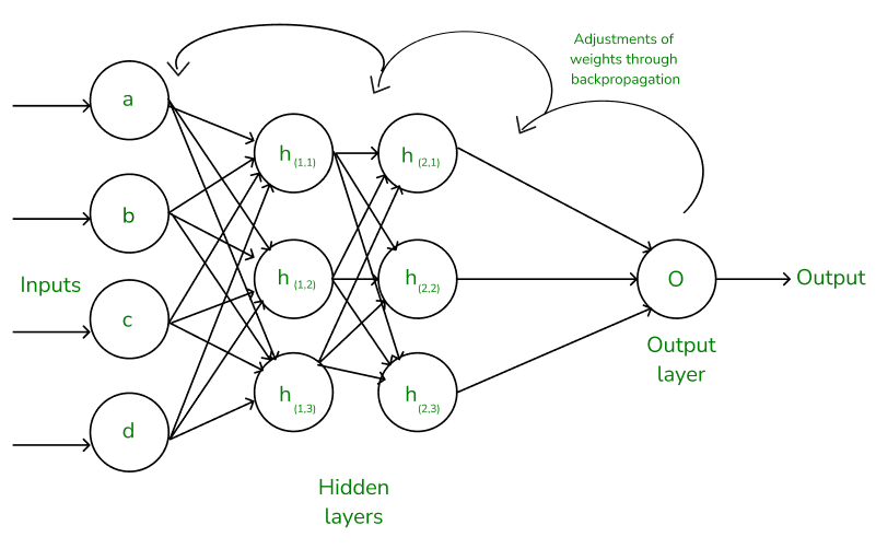
3. Backpropagation:

Backpropagation is the algorithm used to calculate the gradient of the loss function with respect to each weight in the network. This process starts from the output layer and moves backwards through the network, using the chain rule of calculus to compute gradients.

In CNNs, backpropagation needs to handle the unique aspects of convolutional and pooling layers:

• For convolutional layers, the gradient is computed with respect to both the filter weights and the input.
• For pooling layers, the gradient is routed back only through the neuron that was selected in the forward pass (in the case of max pooling).

Source : Geeks for Geeks

4. Optimization:

Once the gradients are computed, an optimization algorithm is used to update the weights of the network. The most commonly used optimizer is Stochastic Gradient Descent (SGD), often with momentum. Other popular optimizers include:

• Adam: Adaptive Moment Estimation, which adapts the learning rate for each parameter.
• RMSprop: Root Mean Square Propagation, which also adapts the learning rate.
• Adagrad: Adaptive Gradient Algorithm, which performs larger updates for infrequent parameters.

For better understanding, Read this Article

These optimizers aim to find the global minimum of the loss function in the high-dimensional space of the network's weights.

5. Regularization:

To prevent overfitting, various regularization techniques are often employed during the learning process:

• L1/L2 regularization: Adds a penalty term to the loss function based on the weights' magnitude.
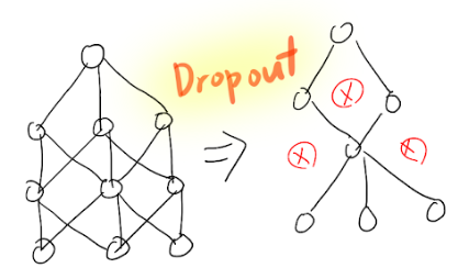
• Dropout: Randomly drops out a proportion of neurons during training, forcing the network to learn more robust features.
• Data augmentation: Artificially increases the training set by applying transformations to the existing data, such as rotations, flips, or color jittering.

6. Batch Normalization:

Batch normalization is a technique that normalizes the inputs to each layer, which can speed up learning and improve generalization. It's typically applied after the convolutional layers and before the activation functions.

For better understanding, Read this article

7. Learning Rate Scheduling:

The learning rate is a crucial hyperparameter that determines the step size during optimization. Learning rate scheduling involves adjusting the learning rate during training, often reducing it over time. Common strategies include:

• Step decay: Reducing the learning rate by a factor at predetermined epochs.
• Exponential decay: Continuously decreasing the learning rate exponentially.
• Cosine annealing: Cyclically varying the learning rate between a maximum and minimum value.

Source : Towards East Asian Facial Expression Recognition in the Real World

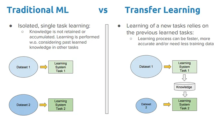
8. Transfer Learning:

In many practical applications, CNNs are not trained from scratch. Instead, transfer learning is used, where a pre-trained model (often trained on a large dataset like ImageNet) is fine-tuned on a specific task. This process typically involves:

• Freezing the early layers of the pre-trained model.
• Replacing and retraining the final layers for the new task.
• Optionally, fine-tuning some of the earlier layers.

Source : Dipanjan (DJ) Sarkar

Understanding the learning process in CNNs is crucial for effectively training and deploying these models. It allows practitioners to make informed decisions about architecture design, hyperparameter tuning, and troubleshooting when things go wrong.

The interplay between these components creates a powerful learning system capable of extracting complex hierarchical features from raw input data. As the field of deep learning continues to evolve, new techniques and refinements to this process are constantly being developed, making it an exciting area of ongoing research.

By mastering these concepts, researchers and practitioners can push the boundaries of what's possible with CNNs, leading to breakthroughs in computer vision, natural language processing, and beyond.