Fully Convolutional Network Overview

1. Introduction to FCN

Fully Convolutional Networks (FCNs) represent a groundbreaking architecture in deep learning, specifically designed for semantic segmentation tasks. Introduced by Long et al. in 2015, FCNs revolutionized the field of computer vision by enabling pixel-wise predictions on input images of arbitrary sizes. Unlike traditional Convolutional Neural Networks (CNNs), FCNs replace fully connected layers with convolutional layers, allowing them to preserve spatial information throughout the network.

The key innovation of FCNs lies in their ability to produce dense predictions for per-pixel tasks like semantic segmentation. This is achieved through a combination of convolutional layers for feature extraction and upsampling techniques to restore the original image resolution. FCNs have found applications in various domains, including autonomous driving, medical image analysis, and satellite imagery interpretation.

Since their inception, FCNs have spawned numerous variants and improvements, each addressing specific challenges in semantic segmentation. Their impact on the field has been profound, setting new benchmarks and inspiring further research into efficient and accurate image segmentation techniques.

2. Structure of FCN

The structure of Fully Convolutional Networks (FCNs) is designed to effectively perform semantic segmentation tasks while maintaining spatial information throughout the network. This section will delve into the key components and architectural details of FCNs.

2.1 Input and Output

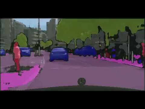
FCNs are capable of processing input images of arbitrary sizes, a significant advantage over traditional CNNs with fixed-size inputs. The input to an FCN is typically a multi-channel image (e.g., RGB), and the output is a segmentation map of the same spatial dimensions as the input, where each pixel is assigned a class label.

Input shape: $(H, W, C)$ Output shape: $(H, W, N)$

Where:

• H: Height of the image
• W: Width of the image
• C: Number of input channels (e.g., 3 for RGB)
• N: Number of classes for segmentation

2.2 Layer Composition

FCNs consist of several key types of layers:

1. Convolutional Layers: These form the backbone of the network, extracting features from the input image. Multiple convolutional layers are stacked to learn hierarchical features.

2. Pooling Layers: Used to reduce spatial dimensions and increase the receptive field. Common types include max pooling and average pooling.

3. Upsampling Layers: These layers restore the spatial dimensions reduced by pooling, typically using transposed convolutions or bilinear interpolation.

4. Skip Connections: These connections combine features from different levels of the network, helping to preserve fine-grained spatial information.

2.3 Network Architecture

A typical FCN architecture can be divided into two main parts:

1. Encoder: This part is similar to a traditional CNN, consisting of convolutional and pooling layers that progressively reduce spatial dimensions while increasing the number of feature channels.

2. Decoder: This part upsamples the feature maps to the original input resolution, often using transposed convolutions or bilinear interpolation.

Here's a simplified representation of an FCN architecture:

Source : ResearchGate

2.4 Skip Connections

Skip connections are a crucial feature of FCNs, allowing the network to combine coarse, semantic information from deeper layers with fine, spatial information from shallower layers. This helps in producing more accurate segmentation boundaries.

A common implementation of skip connections in FCNs is the FCN-8s architecture:

Source : ResearchGate

This architecture combines features from different levels of the network to produce the final segmentation map.

2.5 Loss Function

FCNs typically use pixel-wise cross-entropy loss for training:

$$L = -\frac{1}{N} \sum_{i=1}^N \sum_{c=1}^C y_{ic} \log(\hat{y}_{ic})$$

Where:

• N is the number of pixels
• C is the number of classes
• $y_{ic}$ is the true label for pixel i and class c
• $\hat{y}_{ic}$ is the predicted probability for pixel i and class c

By leveraging this unique structure, FCNs can effectively perform semantic segmentation tasks, producing dense, pixel-wise predictions while maintaining the ability to process images of varying sizes.

3. Operating Principle of FCN

The operating principle of Fully Convolutional Networks (FCNs) is centered around their ability to perform dense prediction tasks, particularly semantic segmentation, by processing an input image through a series of convolutional and upsampling operations. This section will explore the key components and mechanisms that enable FCNs to achieve pixel-wise classification.

3.1 Convolutional Layers

Convolutional layers form the backbone of FCNs, responsible for extracting hierarchical features from the input image. These layers apply a set of learnable filters to the input, producing feature maps that capture various aspects of the image content.

The convolution operation can be mathematically expressed as:

$$(f * g)(x, y) = \sum_{m=-a}^a \sum_{n=-b}^b f(m,n)g(x-m, y-n)$$

Where:

• $f$ is the input feature map
• $g$ is the convolution kernel
• $(x, y)$ are the coordinates of the output feature map

Convolutional layers in FCNs typically use small kernels (e.g., 3x3 or 5x5) and are applied with stride 1 to preserve spatial resolution. The output of each convolutional layer is passed through a non-linear activation function, commonly ReLU (Rectified Linear Unit):

$$ReLU(x) = max(0, x)$$

3.2 Pooling Layers

Pooling layers are used to reduce the spatial dimensions of feature maps, increasing the receptive field of subsequent layers and promoting translation invariance. The most common type of pooling in FCNs is max pooling, which selects the maximum value within a local neighborhood.

Max pooling operation:

$$y_{ij} = \max_{(p,q) \in R_{ij}} x_{pq}$$

Where $R_{ij}$ is the pooling region corresponding to output $y_{ij}$.

While pooling helps in capturing more abstract features, it also reduces spatial resolution, which needs to be addressed in the upsampling phase.

3.3 Upsampling

Upsampling is a crucial component of FCNs, responsible for restoring the spatial dimensions reduced by pooling layers. The most common upsampling methods in FCNs are:

1. Transposed Convolution: Also known as deconvolution or fractionally-strided convolution, this operation learns to upsample feature maps.

2. Bilinear Interpolation: A fixed (non-learnable) upsampling method that computes new pixel values through linear interpolation.

The transposed convolution operation can be expressed as:

$$y = f(W^T * x + b)$$

Where:

• $W^T$ is the transposed weight matrix
• $x$ is the input feature map
• $b$ is the bias term
• $f$ is an activation function

3.4 Skip Connections

Skip connections are a key feature of FCNs, allowing the network to combine high-level semantic information from deeper layers with low-level spatial information from shallower layers. This helps in producing more accurate segmentation boundaries.

The feature fusion in skip connections can be represented as:

$$F_{fused} = F_{deep} \oplus F_{shallow}$$

Where $\oplus$ represents element-wise addition or concatenation.

3.5 End-to-End Training

FCNs are trained end-to-end using backpropagation. The loss function typically used is pixel-wise cross-entropy:

$$L = -\frac{1}{N} \sum_{i=1}^N \sum_{c=1}^C y_{ic} \log(\hat{y}_{ic})$$

Where:

• $N$ is the number of pixels
• $C$ is the number of classes
• $y_{ic}$ is the true label for pixel i and class c
• $\hat{y}_{ic}$ is the predicted probability for pixel i and class c

The network parameters are updated using gradient descent or its variants to minimize this loss function.

By combining these components and principles, FCNs can effectively process input images and produce dense, pixel-wise predictions for semantic segmentation tasks. The ability to preserve spatial information throughout the network, coupled with the use of skip connections and upsampling, allows FCNs to achieve high accuracy in segmentation tasks across various domains.

4. Advantages and Limitations of FCN

Fully Convolutional Networks (FCNs) have significantly impacted the field of semantic segmentation, offering several advantages while also facing certain limitations. This section explores both aspects, providing insights into the strengths and challenges of FCN architecture.

Advantages

1. Pixel-wise Prediction: FCNs enable dense, pixel-level predictions, allowing for precise semantic segmentation of images. This granular prediction capability is crucial for applications requiring detailed spatial understanding, such as autonomous driving and medical image analysis.

2. Spatial Information Preservation: Unlike traditional CNNs with fully connected layers, FCNs maintain spatial information throughout the network. This preservation of spatial context is essential for accurate segmentation, especially at object boundaries.

3. Variable Input Size: FCNs can handle input images of arbitrary sizes, providing flexibility in real-world applications where image dimensions may vary.

4. End-to-end Learning: The entire network can be trained in an end-to-end manner, simplifying the training process and potentially leading to better overall performance.

5. Computational Efficiency: By replacing fully connected layers with convolutional layers, FCNs reduce the number of parameters and computational requirements, especially for large input sizes.

Limitations

1. Loss of Fine Details: Despite skip connections, FCNs can still struggle with preserving very fine details, particularly in deeper networks where multiple pooling operations are applied.

2. Class Imbalance: In scenarios with significant class imbalance (common in many segmentation tasks), FCNs may struggle to accurately predict under-represented classes.

3. Contextual Understanding: While FCNs capture local context well, they may sometimes lack in understanding broader contextual information, which can be crucial for certain segmentation tasks.

4. Boundary Precision: FCNs can sometimes produce segmentation maps with blurry or imprecise object boundaries, especially in complex scenes with multiple overlapping objects.

5. Resolution Trade-off: There's often a trade-off between the depth of the network (which affects the receptive field and semantic understanding) and the preservation of high-resolution details.

To address these limitations, several extensions and modifications to the basic FCN architecture have been proposed:

• U-Net: Incorporates more extensive skip connections to better preserve fine details.
• DeepLab: Uses atrous (dilated) convolutions to increase the receptive field without losing resolution.
• PSPNet: Employs pyramid pooling to capture context at multiple scales.
• Mask R-CNN: Combines FCN with region proposal networks for instance segmentation.

These advancements continue to push the boundaries of what's possible with FCN-based architectures, addressing many of the initial limitations while building upon the core strengths of the FCN approach.