UNet Overview : Image Segmentation

1. Introduction to U-Net

U-Net is a convolutional neural network architecture designed primarily for biomedical image segmentation. Introduced by Olaf Ronneberger, Philipp Fischer, and Thomas Brox in 2015, U-Net has become a standard in medical imaging due to its ability to deliver precise segmentation results with limited training data. The architecture is named "U-Net" because of its U-shaped structure, which symmetrically combines a contracting path (encoder) and an expansive path (decoder). This design allows the network to capture both context and spatial information, making it highly effective for tasks where pixel-level accuracy is crucial. Initially developed for segmenting neuronal structures in electron microscopic stacks, U-Net's versatility has led to its application across various domains, including satellite imagery and autonomous driving. The key innovation of U-Net lies in its use of skip connections that transfer fine-grained features from the encoder to the decoder, preserving spatial resolution and improving segmentation accuracy.

2. Structure of U-Net

The structure of U-Net is ingeniously designed to perform high-precision image segmentation by combining a contracting path with an expansive path. This section delves into the architectural components and their roles in the network.

2.1 Network Architecture

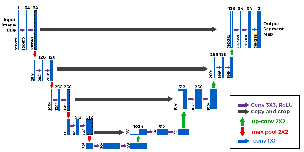
U-Net consists of two main parts: an encoder (contracting path) and a decoder (expansive path), forming a symmetric U-shape.

• Encoder: The encoder is responsible for capturing context through a series of convolutional and pooling layers. It progressively reduces the spatial dimensions while increasing the depth of feature maps, allowing the network to learn complex features at multiple scales.

• Decoder: The decoder upsamples the feature maps back to the original input size, reconstructing the spatial dimensions while maintaining learned features. It consists of up-convolution (transposed convolution) layers that increase spatial resolution.

2.2 Encoder and Decoder

Encoder

The encoder path follows a typical CNN architecture with repeated application of two 3x3 convolutions (unpadded), each followed by a ReLU activation and a 2x2 max pooling operation with stride 2 for downsampling. At each downsampling step, the number of feature channels is doubled.

Decoder

The decoder path involves upsampling the feature map followed by a 2x2 up-convolution that halves the number of feature channels. This is followed by concatenation with the corresponding feature map from the encoder path via skip connections, and two 3x3 convolutions, each followed by a ReLU activation.

2.3 Skip Connections

Skip connections are critical in U-Net's architecture as they directly link corresponding layers between the encoder and decoder paths. These connections allow high-resolution features from early layers in the encoder to be combined with upsampled features in the decoder, preserving spatial information that might otherwise be lost during downsampling.

Source : Geeks for Geeks

2.4 Architectural Details

Layer Type	Operation	Output Size
Input	-	H x W x C
Conv + ReLU	3x3 Convolution	H x W x F
Max Pooling	2x2 Pooling	H/2 x W/2 x F
Up-conv	Transposed Conv	H x W x F/2
Concatenation	Skip Connection	H x W x F
Output	Softmax Activation	H x W x N (Classes)

This architecture allows U-Net to excel in tasks requiring detailed segmentation by effectively combining local features with global context through its unique design.

3. Operating Principle of U-Net

U-Net operates on the principle of combining convolutional operations with strategic upsampling and skip connections to achieve precise image segmentation. This section explores how these components work together to enable effective segmentation.

3.1 Convolution and Upsampling

U-Net employs convolutional layers to extract hierarchical features from input images. Each convolutional layer applies multiple filters to capture various patterns within local regions of the image:

$$(f * g)(x, y) = \sum_{m=-a}^a \sum_{n=-b}^b f(m,n)g(x-m, y-n)$$

Where:

• $f$ is the input feature map
• $g$ is the convolution kernel
• $(x, y)$ are coordinates on the output feature map

In contrast, upsampling layers in U-Net restore spatial dimensions reduced during encoding using transposed convolutions:

$$y = f(W^T * x + b)$$

Where:

• $W^T$ is the transposed weight matrix
• $x$ is the input feature map
• $b$ is bias
• $f$ is an activation function such as ReLU

3.2 Role of Skip Connections

Skip connections are pivotal in maintaining high-resolution details throughout U-Net's processing pipeline. By concatenating high-resolution features from early layers in the encoder with corresponding upsampled features in the decoder, skip connections ensure that fine-grained spatial information is preserved:

$$F_{fused} = F_{deep} \oplus F_{shallow}$$

Where $\oplus$ represents element-wise addition or concatenation.

3.3 Loss Function and Training Process

U-Net typically uses a pixel-wise cross-entropy loss function for training, which measures discrepancies between predicted segmentation maps and ground truth labels:

$$L = -\frac{1}{N} \sum_{i=1}^N \sum_{c=1}^C y_{ic} \log(\hat{y}_{ic})$$

Where:

• $N$ is total pixels
• $C$ is number of classes
• $y_{ic}$ is true label for pixel i and class c
• $\hat{y}_{ic}$ is predicted probability for pixel i and class c

During training, backpropagation adjusts network weights to minimize this loss function using gradient descent or its variants.

3.4 End-to-End Learning

U-Net's end-to-end learning capability allows it to learn optimal feature representations directly from raw data without requiring manual feature engineering. This approach enables rapid adaptation across diverse datasets while maintaining high accuracy levels.

By integrating these principles into its architecture, U-Net achieves state-of-the-art performance across various domains requiring detailed image segmentation—demonstrating remarkable versatility despite being initially designed for biomedical applications alone.

4. Advantages and Limitations of U-Net

Advantages

1. High Precision: U-Net excels at providing detailed pixel-level segmentation due to its unique architecture combining convolutional operations with skip connections.

2. Data Efficiency: It performs well even on small datasets thanks to extensive data augmentation strategies employed during training.

3. Versatility: Originally developed for biomedical applications; however; it has been successfully applied across numerous fields including satellite imagery analysis & autonomous driving systems.

Limitations

1. Computational Demand: Despite efficiency improvements over traditional CNNs; large-scale implementations still require significant computational resources—particularly when dealing with high-resolution images.

2. Boundary Precision: Although improved compared to earlier models; boundary precision remains challenging—especially when segmenting complex structures or overlapping objects within scenes.

5. Variants and Developments of U-Net

U-Net has inspired several variants aimed at enhancing its performance across different applications:

1. 3D U-Net: Extends original model into three dimensions—enabling volumetric segmentation tasks such as MRI scans or CT images.

2. Attention U-Net: Incorporates attention mechanisms into existing framework—allowing model focus selectively on relevant regions within input images while ignoring irrelevant background noise.

3. Residual U-Net: Combines residual learning techniques with traditional u-shaped architecture—improving convergence speed & overall accuracy levels during training process.

These advancements continue pushing boundaries beyond initial capabilities set forth by original design—demonstrating ongoing evolution within field driven largely by real-world demands faced daily across industries worldwide!